1.Gaussian Mixture Models(GMM)
For a D-dimensional feature vector, x, the mixture density used for the likelihood function is defined as
$p(x|\lambda) = \sum_{i=1}^{M}w_{i}p_{i}(x)$.
The density is a weighted linear combination of $M$ unimodal Gaussian densities , $p_{i}(x)$
$p_{i}(x) = \frac{1}{(2\pi)^{D/2}|\sum _{i}|^{1/2}} exp[-\frac{1}{2}(x-\mu_{i})^{T}(\sum _{i})^{-1}(x-\mu_{i})]$.
2.Support Vector Machines(SVM)
An SVM is a two-class classifier constructed from sums of a kernel function $K(• , •)$
$f(x) = \sum_{i=1}{N}\alpha_{i} t_{i} K(x,x_{i}) + d$.
$t_{i}$ are the ideal outputs, $\sum_{i=1}{N}\alpha_{i} t_{i}=0$ and $\alpha_{i} > 0$,$x_{i}$ are support vectors and obtained
from the training set by an optimization process.
$K(. , .)$ is constrained to have certain properties (the Mercer condition), so that it can be expressed as
$K(x,y) = b(x)^{T} b(y)$.
Kernel function examples:
http://www.shamoxia.com/html/y2010/2292.html
3.GMM-SVM
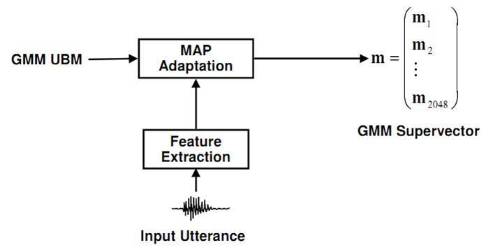
GMM Supervectors:given a speaker utterance, GMM-UBM training is performed by MAP adaptation of the means $m_{i}$,
and we form a GMM supervector $m = [m_{i}]$
 GMM Supervectors Linear Kernel: a natural distance between the two utterances is the KL divergence, while it does n't satisfy
the Mercer condition, we consider the following approximation
$\begin{align}
D(g_{a}\parallel g_{b}) = &\int_{R^{n}}g_{a}xlog\left(\frac{g_{a}(x)}{g_{b}(x)} \right)dx \\
\leq & \sum_{i=1}^{N} \lambda _{i}D(N(.;m_{i}^{a},\Sigma _{i})\parallel N(.;m_{i}^{b},\Sigma _{i}))\\
= &\frac{1}{2}\sum_{i=1}^{N}\lambda_{i}(m_{i}^{a}-m_{i}^{b})\Sigma ^{-1}(m_{i}^{a}-m_{i}^{b})
\end{align}$
we can define a new distance formula,
$d(m^{a},m^{b}) = \frac{1}{2} \sum_{i=1}^{N}\lambda_{i}(m_{i}^{a}-m_{i}^{b})\Sigma_{i}^{-1}(m_{i}^{a}-m_{i}^{b})$
From the distance, we can find the corresponding inner product which is the kernel function.
4.SVM-NAP
Nuisance Attribute Projection(NAP) attempts to remove the unwanted within-class variation of the observed feature vectors.
This is achieved by applying the transform
$y' = P_{n}y = (I-V_{n}V_{n}^{T})y$.
where Vn is the principal directions of within-class variability.
The SVM NAP constructs a new kernel,
$\begin{align}
K(m^{a},m^{b}) =& [Pb(m^{a})]^{T}[Pb(m^{b})]\\
=& b(m^{a})^{t}Pb(m^{b})\\
=& b(m^{a})^{t}(I-vv^{t})b(m^{b})
\end{align}$.
where $P$ is a projection ($P^{2} = P$) , $v$ is the direction being removed from the SVM expansion
space. $b(.)$ is the SVM expansion, and $\parallel v\parallel ^{2} = 1$.
5.Experiments on NIST SRE 2010
In the experiments, I use the spro4 to extract MFCC and LPCC features, and use Alize to
build GMM-UBM and all of the remained tasks.
References
[1]Douglas A. Reynolds, T. F. Quatieri, and R. Dunn, Speaker verication using adapted Gaussian mixture models, Digital Signal Processing, vol. 10, no. 1-3, pp. 1941, 2000.
[2]W. Campbell, “Generalized linear discriminant sequence kernels for speaker recognition,” in IEEE International Conference on Acoustics, Speech, and Signal Processing, vol. 1, 2002, pp. 161–164.
[3]W. M. Campbell, D. E. Sturim, D. A. Reynolds, A. Solomonoff, SVM Based Speaker Verification Using a GMM Supervector Kernel and NAP Variability Compensation.
[4]Robbie Vogt, Sachin Kajarekar, Sridha Sridharan, Discriminant NAP for SVM Speaker Recognition.
 GMM Supervectors Linear Kernel: a natural distance between the two utterances is the KL divergence, while it does n't satisfy
the Mercer condition, we consider the following approximation